import numpy as np
import pandas as pd
inputfile = '../data/data.csv'
data = pd.read_csv(inputfile)
description = [data.min(), data.max(), data.mean(),
data.std()]
description = pd.DataFrame(
description, index=['Min', 'Max', 'Mean', 'STD']).T
print('描述性统计结果:\n', np.round(description, 2))
描述性统计结果:
             Min         Max        Mean         STD
x1   3831732.00  7599295.00  5579519.95  1262194.72
x2       181.54     2110.78      765.04      595.70
x3       448.19     6882.85     2370.83     1919.17
x4      7571.00    42049.14    19644.69    10203.02
x5      6212.70    33156.83    15870.95     8199.77
x6   6370241.00  8323096.00  7350513.60   621341.85
x7       525.71     4454.55     1712.24     1184.71
x8       985.31    15420.14     5705.80     4478.40
x9        60.62      228.46      129.49       50.51
x10       65.66      852.56      340.22      251.58
x11       97.50      120.00      103.31        5.51
x12        1.03        1.91        1.42        0.25
x13     5321.00    41972.00    17273.80    11109.19
y         64.87     2088.14      618.08      609.25
corr = data.corr(method='pearson')
print('相关系数矩阵为:\n', np.round(corr, 2))
相关系数矩阵为:
        x1    x2    x3    x4    x5    x6    x7    x8    x9   x10   x11   x12  \
x1   1.00  0.95  0.95  0.97  0.97  0.99  0.95  0.97  0.98  0.98 -0.29  0.94
x2   0.95  1.00  1.00  0.99  0.99  0.92  0.99  0.99  0.98  0.98 -0.13  0.89
x3   0.95  1.00  1.00  0.99  0.99  0.92  1.00  0.99  0.98  0.99 -0.15  0.89
x4   0.97  0.99  0.99  1.00  1.00  0.95  0.99  1.00  0.99  1.00 -0.19  0.91
x5   0.97  0.99  0.99  1.00  1.00  0.95  0.99  1.00  0.99  1.00 -0.18  0.90
x6   0.99  0.92  0.92  0.95  0.95  1.00  0.93  0.95  0.97  0.96 -0.34  0.95
x7   0.95  0.99  1.00  0.99  0.99  0.93  1.00  0.99  0.98  0.99 -0.15  0.89
x8   0.97  0.99  0.99  1.00  1.00  0.95  0.99  1.00  0.99  1.00 -0.15  0.90
x9   0.98  0.98  0.98  0.99  0.99  0.97  0.98  0.99  1.00  0.99 -0.23  0.91
x10  0.98  0.98  0.99  1.00  1.00  0.96  0.99  1.00  0.99  1.00 -0.17  0.90
x11 -0.29 -0.13 -0.15 -0.19 -0.18 -0.34 -0.15 -0.15 -0.23 -0.17  1.00 -0.43
x12  0.94  0.89  0.89  0.91  0.90  0.95  0.89  0.90  0.91  0.90 -0.43  1.00
x13  0.96  1.00  1.00  1.00  0.99  0.94  1.00  1.00  0.99  0.99 -0.16  0.90
y    0.94  0.98  0.99  0.99  0.99  0.91  0.99  0.99  0.98  0.99 -0.12  0.87

      x13     y
x1   0.96  0.94
x2   1.00  0.98
x3   1.00  0.99
x4   1.00  0.99
x5   0.99  0.99
x6   0.94  0.91
x7   1.00  0.99
x8   1.00  0.99
x9   0.99  0.98
x10  0.99  0.99
x11 -0.16 -0.12
x12  0.90  0.87
x13  1.00  0.99
y    0.99  1.00
import matplotlib.pyplot as plt
import seaborn as sns
plt.rcParams['font.sans-serif'] = ['SimHei']
plt.rcParams['axes.unicode_minus'] = False
plt.subplots(figsize=(12, 12))
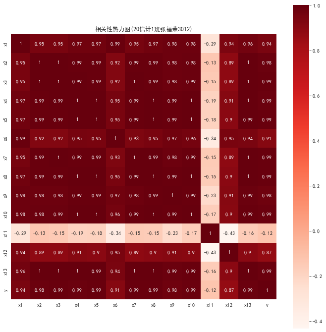
sns.heatmap(corr, annot=True, vmax=1, square=True, cmap="Reds")
plt.title('相关性热力图(20信计1班李之琛3322)')
plt.savefig('../imag/hot.jpg', dpi=600)
plt.show()
import matplotlib.pyplot as plt
import seaborn as sns
plt.rcParams['font.sans-serif'] = ['SimHei']
plt.rcParams['axes.unicode_minus'] = False
plt.subplots(figsize=(10, 10))
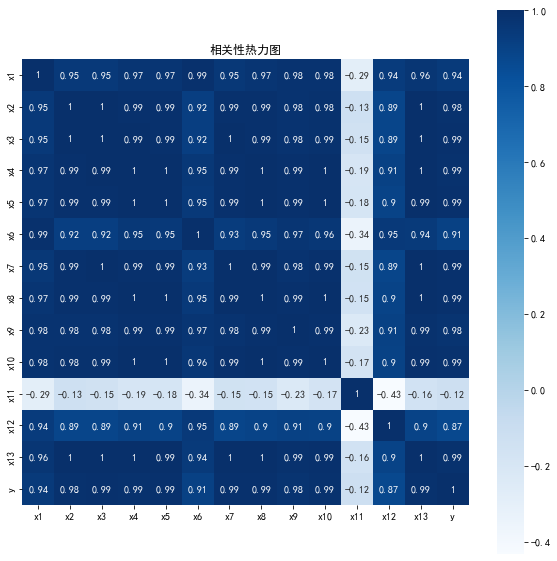
sns.heatmap(corr, annot=True, vmax=1, square=True, cmap="Blues")
plt.title('相关性热力图')
plt.show()
import numpy as np
import pandas as pd
from sklearn.linear_model import Lasso
inputfile = '../data/data.csv'
data = pd.read_csv(inputfile)
lasso = Lasso(1000)
lasso.fit(data.iloc[:,0:13],data['y'])
print('相关系数为:',np.round(lasso.coef_,5))
相关系数为: [-1.8000e-04 -0.0000e+00  1.2414e-01 -1.0310e-02  6.5400e-02  1.2000e-04
  3.1741e-01  3.4900e-02 -0.0000e+00  0.0000e+00  0.0000e+00  0.0000e+00
 -4.0300e-02]


F:\Anaconda\envs\my\lib\site-packages\sklearn\linear_model\_coordinate_descent.py:648: ConvergenceWarning: Objective did not converge. You might want to increase the number of iterations, check the scale of the features or consider increasing regularisation. Duality gap: 3.417e+04, tolerance: 7.053e+02
  model = cd_fast.enet_coordinate_descent(
lasso.coef_
array([-1.76147790e-04, -0.00000000e+00,  1.24143041e-01, -1.03120575e-02,
        6.53999569e-02,  1.15234764e-04,  3.17411469e-01,  3.49002210e-02,
       -0.00000000e+00,  0.00000000e+00,  0.00000000e+00,  0.00000000e+00,
       -4.02991430e-02])
print('相关系数非零个数为:',np.sum(lasso.coef_ != 0))
相关系数非零个数为: 8
mask = lasso.coef_ != 0
print('相关系数是否为零:',mask)
相关系数是否为零: [ True False  True  True  True  True  True  True False False False False
  True]
data.head(5)
| x1 | x2 | x3 | x4 | x5 | x6 | x7 | x8 | x9 | x10 | x11 | x12 | x13 | y |
|---|
| 0 | 3831732 | 181.54 | 448.19 | 7571.00 | 6212.70 | 6370241 | 525.71 | 985.31 | 60.62 | 65.66 | 120.0 | 1.029 | 5321 | 64.87 |
|---|
| 1 | 3913824 | 214.63 | 549.97 | 9038.16 | 7601.73 | 6467115 | 618.25 | 1259.20 | 73.46 | 95.46 | 113.5 | 1.051 | 6529 | 99.75 |
|---|
| 2 | 3928907 | 239.56 | 686.44 | 9905.31 | 8092.82 | 6560508 | 638.94 | 1468.06 | 81.16 | 81.16 | 108.2 | 1.064 | 7008 | 88.11 |
|---|
| 3 | 4282130 | 261.58 | 802.59 | 10444.60 | 8767.98 | 6664862 | 656.58 | 1678.12 | 85.72 | 91.70 | 102.2 | 1.092 | 7694 | 106.07 |
|---|
| 4 | 4453911 | 283.14 | 904.57 | 11255.70 | 9422.33 | 6741400 | 758.83 | 1893.52 | 88.88 | 114.61 | 97.7 | 1.200 | 8027 | 137.32 |
|---|
mask = np.append(mask,True)
mask
array([ True, False,  True,  True,  True,  True,  True,  True, False,
       False, False, False,  True,  True])
outputfile ='../tmp/new_reg_data_2.csv'
new_reg_data = data.iloc[:, mask]
new_reg_data
| x1 | x3 | x4 | x5 | x6 | x7 | x8 | x13 | y |
|---|
| 0 | 3831732 | 448.19 | 7571.00 | 6212.70 | 6370241 | 525.71 | 985.31 | 5321 | 64.87 |
|---|
| 1 | 3913824 | 549.97 | 9038.16 | 7601.73 | 6467115 | 618.25 | 1259.20 | 6529 | 99.75 |
|---|
| 2 | 3928907 | 686.44 | 9905.31 | 8092.82 | 6560508 | 638.94 | 1468.06 | 7008 | 88.11 |
|---|
| 3 | 4282130 | 802.59 | 10444.60 | 8767.98 | 6664862 | 656.58 | 1678.12 | 7694 | 106.07 |
|---|
| 4 | 4453911 | 904.57 | 11255.70 | 9422.33 | 6741400 | 758.83 | 1893.52 | 8027 | 137.32 |
|---|
| 5 | 4548852 | 1000.69 | 12018.52 | 9751.44 | 6850024 | 878.26 | 2139.18 | 8549 | 188.14 |
|---|
| 6 | 4962579 | 1121.13 | 13966.53 | 11349.47 | 7006896 | 923.67 | 2492.74 | 9566 | 219.91 |
|---|
| 7 | 5029338 | 1248.29 | 14694.00 | 11467.35 | 7125979 | 978.21 | 2841.65 | 10473 | 271.91 |
|---|
| 8 | 5070216 | 1370.68 | 13380.47 | 10671.78 | 7206229 | 1009.24 | 3203.96 | 11469 | 269.10 |
|---|
| 9 | 5210706 | 1494.27 | 15002.59 | 11570.58 | 7251888 | 1175.17 | 3758.62 | 12360 | 300.55 |
|---|
| 10 | 5407087 | 1677.77 | 16884.16 | 13120.83 | 7376720 | 1348.93 | 4450.55 | 14174 | 338.45 |
|---|
| 11 | 5744550 | 1905.84 | 18287.24 | 14468.24 | 7505322 | 1519.16 | 5154.23 | 16394 | 408.86 |
|---|
| 12 | 5994973 | 2199.14 | 19850.66 | 15444.93 | 7607220 | 1696.38 | 6081.86 | 17881 | 476.72 |
|---|
| 13 | 6236312 | 2624.24 | 22469.22 | 18951.32 | 7734787 | 1863.34 | 7140.32 | 20058 | 838.99 |
|---|
| 14 | 6529045 | 3187.39 | 25316.72 | 20835.95 | 7841695 | 2105.54 | 8287.38 | 22114 | 843.14 |
|---|
| 15 | 6791495 | 3615.77 | 27609.59 | 22820.89 | 7946154 | 2659.85 | 9138.21 | 24190 | 1107.67 |
|---|
| 16 | 7110695 | 4476.38 | 30658.49 | 25011.61 | 8061370 | 3263.57 | 10748.28 | 29549 | 1399.16 |
|---|
| 17 | 7431755 | 5243.03 | 34438.08 | 28209.74 | 8145797 | 3412.21 | 12423.44 | 34214 | 1535.14 |
|---|
| 18 | 7512997 | 5977.27 | 38053.52 | 30490.44 | 8222969 | 3758.39 | 13551.21 | 37934 | 1579.68 |
|---|
| 19 | 7599295 | 6882.85 | 42049.14 | 33156.83 | 8323096 | 4454.55 | 15420.14 | 41972 | 2088.14 |
|---|
new_reg_data = new_reg_data.iloc[:,:-1]
new_reg_data
| x1 | x3 | x4 | x5 | x6 | x7 | x8 | x13 |
|---|
| 0 | 3831732 | 448.19 | 7571.00 | 6212.70 | 6370241 | 525.71 | 985.31 | 5321 |
|---|
| 1 | 3913824 | 549.97 | 9038.16 | 7601.73 | 6467115 | 618.25 | 1259.20 | 6529 |
|---|
| 2 | 3928907 | 686.44 | 9905.31 | 8092.82 | 6560508 | 638.94 | 1468.06 | 7008 |
|---|
| 3 | 4282130 | 802.59 | 10444.60 | 8767.98 | 6664862 | 656.58 | 1678.12 | 7694 |
|---|
| 4 | 4453911 | 904.57 | 11255.70 | 9422.33 | 6741400 | 758.83 | 1893.52 | 8027 |
|---|
| 5 | 4548852 | 1000.69 | 12018.52 | 9751.44 | 6850024 | 878.26 | 2139.18 | 8549 |
|---|
| 6 | 4962579 | 1121.13 | 13966.53 | 11349.47 | 7006896 | 923.67 | 2492.74 | 9566 |
|---|
| 7 | 5029338 | 1248.29 | 14694.00 | 11467.35 | 7125979 | 978.21 | 2841.65 | 10473 |
|---|
| 8 | 5070216 | 1370.68 | 13380.47 | 10671.78 | 7206229 | 1009.24 | 3203.96 | 11469 |
|---|
| 9 | 5210706 | 1494.27 | 15002.59 | 11570.58 | 7251888 | 1175.17 | 3758.62 | 12360 |
|---|
| 10 | 5407087 | 1677.77 | 16884.16 | 13120.83 | 7376720 | 1348.93 | 4450.55 | 14174 |
|---|
| 11 | 5744550 | 1905.84 | 18287.24 | 14468.24 | 7505322 | 1519.16 | 5154.23 | 16394 |
|---|
| 12 | 5994973 | 2199.14 | 19850.66 | 15444.93 | 7607220 | 1696.38 | 6081.86 | 17881 |
|---|
| 13 | 6236312 | 2624.24 | 22469.22 | 18951.32 | 7734787 | 1863.34 | 7140.32 | 20058 |
|---|
| 14 | 6529045 | 3187.39 | 25316.72 | 20835.95 | 7841695 | 2105.54 | 8287.38 | 22114 |
|---|
| 15 | 6791495 | 3615.77 | 27609.59 | 22820.89 | 7946154 | 2659.85 | 9138.21 | 24190 |
|---|
| 16 | 7110695 | 4476.38 | 30658.49 | 25011.61 | 8061370 | 3263.57 | 10748.28 | 29549 |
|---|
| 17 | 7431755 | 5243.03 | 34438.08 | 28209.74 | 8145797 | 3412.21 | 12423.44 | 34214 |
|---|
| 18 | 7512997 | 5977.27 | 38053.52 | 30490.44 | 8222969 | 3758.39 | 13551.21 | 37934 |
|---|
| 19 | 7599295 | 6882.85 | 42049.14 | 33156.83 | 8323096 | 4454.55 | 15420.14 | 41972 |
|---|
new_reg_data.to_csv(outputfile)
print('输出数据的维度为:',new_reg_data.shape)
输出数据的维度为: (20, 8)
def GM11(x0):
import numpy as np
x1 = x0.cumsum()
z1 = (x1[:len(x1)-1] + x1[1:])/2.0
z1 = z1.reshape((len(z1),1))
B = np.append(-z1, np.ones_like(z1), axis = 1)
Yn = x0[1:].reshape((len(x0)-1, 1))
[[a],[b]] = np.dot(np.dot(np.linalg.inv(np.dot(B.T, B)), B.T), Yn)
f = lambda k: (x0[0]-b/a)*np.exp(-a*(k-1))-(x0[0]-b/a)*np.exp(-a*(k-2))
delta = np.abs(x0 - np.array([f(i) for i in range(1,len(x0)+1)]))
C = delta.std()/x0.std()
P = 1.0*(np.abs(delta - delta.mean()) < 0.6745*x0.std()).sum()/len(x0)
return f, a, b, x0[0], C, P
import numpy as np
import pandas as pd
inputfile1 = '../tmp/new_reg_data_2.csv'
inputfile2 = '../data/data.csv'
new_reg_data = pd.read_csv(inputfile1)
data = pd.read_csv(inputfile2)
new_reg_data.index = range(1994, 2014)
new_reg_data.loc[2014] = None
new_reg_data.loc[2015] = None
l = ['x1', 'x3', 'x4', 'x5', 'x6', 'x7', 'x8', 'x13']
C:\Windows\Temp\ipykernel_63584\756966604.py:6: FutureWarning: The default dtype for empty Series will be 'object' instead of 'float64' in a future version. Specify a dtype explicitly to silence this warning.
  new_reg_data.loc[2014] = None
C:\Windows\Temp\ipykernel_63584\756966604.py:7: FutureWarning: The default dtype for empty Series will be 'object' instead of 'float64' in a future version. Specify a dtype explicitly to silence this warning.
  new_reg_data.loc[2015] = None
new_reg_data
| Unnamed: 0 | x1 | x3 | x4 | x5 | x6 | x7 | x8 | x13 |
|---|
| 1994 | 0.0 | 3831732.0 | 448.19 | 7571.00 | 6212.70 | 6370241.0 | 525.71 | 985.31 | 5321.0 |
|---|
| 1995 | 1.0 | 3913824.0 | 549.97 | 9038.16 | 7601.73 | 6467115.0 | 618.25 | 1259.20 | 6529.0 |
|---|
| 1996 | 2.0 | 3928907.0 | 686.44 | 9905.31 | 8092.82 | 6560508.0 | 638.94 | 1468.06 | 7008.0 |
|---|
| 1997 | 3.0 | 4282130.0 | 802.59 | 10444.60 | 8767.98 | 6664862.0 | 656.58 | 1678.12 | 7694.0 |
|---|
| 1998 | 4.0 | 4453911.0 | 904.57 | 11255.70 | 9422.33 | 6741400.0 | 758.83 | 1893.52 | 8027.0 |
|---|
| 1999 | 5.0 | 4548852.0 | 1000.69 | 12018.52 | 9751.44 | 6850024.0 | 878.26 | 2139.18 | 8549.0 |
|---|
| 2000 | 6.0 | 4962579.0 | 1121.13 | 13966.53 | 11349.47 | 7006896.0 | 923.67 | 2492.74 | 9566.0 |
|---|
| 2001 | 7.0 | 5029338.0 | 1248.29 | 14694.00 | 11467.35 | 7125979.0 | 978.21 | 2841.65 | 10473.0 |
|---|
| 2002 | 8.0 | 5070216.0 | 1370.68 | 13380.47 | 10671.78 | 7206229.0 | 1009.24 | 3203.96 | 11469.0 |
|---|
| 2003 | 9.0 | 5210706.0 | 1494.27 | 15002.59 | 11570.58 | 7251888.0 | 1175.17 | 3758.62 | 12360.0 |
|---|
| 2004 | 10.0 | 5407087.0 | 1677.77 | 16884.16 | 13120.83 | 7376720.0 | 1348.93 | 4450.55 | 14174.0 |
|---|
| 2005 | 11.0 | 5744550.0 | 1905.84 | 18287.24 | 14468.24 | 7505322.0 | 1519.16 | 5154.23 | 16394.0 |
|---|
| 2006 | 12.0 | 5994973.0 | 2199.14 | 19850.66 | 15444.93 | 7607220.0 | 1696.38 | 6081.86 | 17881.0 |
|---|
| 2007 | 13.0 | 6236312.0 | 2624.24 | 22469.22 | 18951.32 | 7734787.0 | 1863.34 | 7140.32 | 20058.0 |
|---|
| 2008 | 14.0 | 6529045.0 | 3187.39 | 25316.72 | 20835.95 | 7841695.0 | 2105.54 | 8287.38 | 22114.0 |
|---|
| 2009 | 15.0 | 6791495.0 | 3615.77 | 27609.59 | 22820.89 | 7946154.0 | 2659.85 | 9138.21 | 24190.0 |
|---|
| 2010 | 16.0 | 7110695.0 | 4476.38 | 30658.49 | 25011.61 | 8061370.0 | 3263.57 | 10748.28 | 29549.0 |
|---|
| 2011 | 17.0 | 7431755.0 | 5243.03 | 34438.08 | 28209.74 | 8145797.0 | 3412.21 | 12423.44 | 34214.0 |
|---|
| 2012 | 18.0 | 7512997.0 | 5977.27 | 38053.52 | 30490.44 | 8222969.0 | 3758.39 | 13551.21 | 37934.0 |
|---|
| 2013 | 19.0 | 7599295.0 | 6882.85 | 42049.14 | 33156.83 | 8323096.0 | 4454.55 | 15420.14 | 41972.0 |
|---|
| 2014 | NaN | NaN | NaN | NaN | NaN | NaN | NaN | NaN | NaN |
|---|
| 2015 | NaN | NaN | NaN | NaN | NaN | NaN | NaN | NaN | NaN |
|---|
import xlwt
for i in l:
f = GM11(new_reg_data.loc[range(1994, 2014),i].values)[0]
new_reg_data.loc[2014,i] = f(len(new_reg_data)-1)
new_reg_data.loc[2015,i] = f(len(new_reg_data))
new_reg_data[i] = new_reg_data[i].round(2)
outputfile = '../tmp/new_reg_data_GM11_2.xls'
y = list(data['y'].values)
y.extend([np.nan,np.nan])
new_reg_data['y'] = y
new_reg_data.to_excel(outputfile)
print('预测结果为:\n',new_reg_data.loc[2014:2015,:])
预测结果为:
       Unnamed: 0          x1       x3        x4        x5          x6  \
2014         NaN  8142148.24  7042.31  43611.84  35046.63  8505522.58
2015         NaN  8460489.28  8166.92  47792.22  38384.22  8627139.31

           x7        x8       x13   y
2014  4600.40  18686.28  44506.47 NaN
2015  5214.78  21474.47  49945.88 NaN


C:\Windows\Temp\ipykernel_63584\1948140384.py:10: FutureWarning: As the xlwt package is no longer maintained, the xlwt engine will be removed in a future version of pandas. This is the only engine in pandas that supports writing in the xls format. Install openpyxl and write to an xlsx file instead. You can set the option io.excel.xls.writer to 'xlwt' to silence this warning. While this option is deprecated and will also raise a warning, it can be globally set and the warning suppressed.
  new_reg_data.to_excel(outputfile)  # 结果输出
import matplotlib.pyplot as plt
from sklearn.svm import LinearSVR
inputfile = '../tmp/new_reg_data_GM11_2.xls'
data = pd.read_excel(inputfile)
feature = ['x1', 'x3', 'x4', 'x5', 'x6', 'x7', 'x8', 'x13']
data
| Unnamed: 0.1 | Unnamed: 0 | x1 | x3 | x4 | x5 | x6 | x7 | x8 | x13 | y |
|---|
| 0 | 1994 | 0.0 | 3831732.00 | 448.19 | 7571.00 | 6212.70 | 6370241.00 | 525.71 | 985.31 | 5321.00 | 64.87 |
|---|
| 1 | 1995 | 1.0 | 3913824.00 | 549.97 | 9038.16 | 7601.73 | 6467115.00 | 618.25 | 1259.20 | 6529.00 | 99.75 |
|---|
| 2 | 1996 | 2.0 | 3928907.00 | 686.44 | 9905.31 | 8092.82 | 6560508.00 | 638.94 | 1468.06 | 7008.00 | 88.11 |
|---|
| 3 | 1997 | 3.0 | 4282130.00 | 802.59 | 10444.60 | 8767.98 | 6664862.00 | 656.58 | 1678.12 | 7694.00 | 106.07 |
|---|
| 4 | 1998 | 4.0 | 4453911.00 | 904.57 | 11255.70 | 9422.33 | 6741400.00 | 758.83 | 1893.52 | 8027.00 | 137.32 |
|---|
| 5 | 1999 | 5.0 | 4548852.00 | 1000.69 | 12018.52 | 9751.44 | 6850024.00 | 878.26 | 2139.18 | 8549.00 | 188.14 |
|---|
| 6 | 2000 | 6.0 | 4962579.00 | 1121.13 | 13966.53 | 11349.47 | 7006896.00 | 923.67 | 2492.74 | 9566.00 | 219.91 |
|---|
| 7 | 2001 | 7.0 | 5029338.00 | 1248.29 | 14694.00 | 11467.35 | 7125979.00 | 978.21 | 2841.65 | 10473.00 | 271.91 |
|---|
| 8 | 2002 | 8.0 | 5070216.00 | 1370.68 | 13380.47 | 10671.78 | 7206229.00 | 1009.24 | 3203.96 | 11469.00 | 269.10 |
|---|
| 9 | 2003 | 9.0 | 5210706.00 | 1494.27 | 15002.59 | 11570.58 | 7251888.00 | 1175.17 | 3758.62 | 12360.00 | 300.55 |
|---|
| 10 | 2004 | 10.0 | 5407087.00 | 1677.77 | 16884.16 | 13120.83 | 7376720.00 | 1348.93 | 4450.55 | 14174.00 | 338.45 |
|---|
| 11 | 2005 | 11.0 | 5744550.00 | 1905.84 | 18287.24 | 14468.24 | 7505322.00 | 1519.16 | 5154.23 | 16394.00 | 408.86 |
|---|
| 12 | 2006 | 12.0 | 5994973.00 | 2199.14 | 19850.66 | 15444.93 | 7607220.00 | 1696.38 | 6081.86 | 17881.00 | 476.72 |
|---|
| 13 | 2007 | 13.0 | 6236312.00 | 2624.24 | 22469.22 | 18951.32 | 7734787.00 | 1863.34 | 7140.32 | 20058.00 | 838.99 |
|---|
| 14 | 2008 | 14.0 | 6529045.00 | 3187.39 | 25316.72 | 20835.95 | 7841695.00 | 2105.54 | 8287.38 | 22114.00 | 843.14 |
|---|
| 15 | 2009 | 15.0 | 6791495.00 | 3615.77 | 27609.59 | 22820.89 | 7946154.00 | 2659.85 | 9138.21 | 24190.00 | 1107.67 |
|---|
| 16 | 2010 | 16.0 | 7110695.00 | 4476.38 | 30658.49 | 25011.61 | 8061370.00 | 3263.57 | 10748.28 | 29549.00 | 1399.16 |
|---|
| 17 | 2011 | 17.0 | 7431755.00 | 5243.03 | 34438.08 | 28209.74 | 8145797.00 | 3412.21 | 12423.44 | 34214.00 | 1535.14 |
|---|
| 18 | 2012 | 18.0 | 7512997.00 | 5977.27 | 38053.52 | 30490.44 | 8222969.00 | 3758.39 | 13551.21 | 37934.00 | 1579.68 |
|---|
| 19 | 2013 | 19.0 | 7599295.00 | 6882.85 | 42049.14 | 33156.83 | 8323096.00 | 4454.55 | 15420.14 | 41972.00 | 2088.14 |
|---|
| 20 | 2014 | NaN | 8142148.24 | 7042.31 | 43611.84 | 35046.63 | 8505522.58 | 4600.40 | 18686.28 | 44506.47 | NaN |
|---|
| 21 | 2015 | NaN | 8460489.28 | 8166.92 | 47792.22 | 38384.22 | 8627139.31 | 5214.78 | 21474.47 | 49945.88 | NaN |
|---|
data_train=data.loc[0:19,:]
data_train.head()
| Unnamed: 0.1 | Unnamed: 0 | x1 | x3 | x4 | x5 | x6 | x7 | x8 | x13 | y |
|---|
| 0 | 1994 | 0.0 | 3831732.0 | 448.19 | 7571.00 | 6212.70 | 6370241.0 | 525.71 | 985.31 | 5321.0 | 64.87 |
|---|
| 1 | 1995 | 1.0 | 3913824.0 | 549.97 | 9038.16 | 7601.73 | 6467115.0 | 618.25 | 1259.20 | 6529.0 | 99.75 |
|---|
| 2 | 1996 | 2.0 | 3928907.0 | 686.44 | 9905.31 | 8092.82 | 6560508.0 | 638.94 | 1468.06 | 7008.0 | 88.11 |
|---|
| 3 | 1997 | 3.0 | 4282130.0 | 802.59 | 10444.60 | 8767.98 | 6664862.0 | 656.58 | 1678.12 | 7694.0 | 106.07 |
|---|
| 4 | 1998 | 4.0 | 4453911.0 | 904.57 | 11255.70 | 9422.33 | 6741400.0 | 758.83 | 1893.52 | 8027.0 | 137.32 |
|---|
data_mean = data_train.mean()
data_std = data_train.std()
data_train = (data_train - data_mean)/data_std
x_train = data_train[feature].values
y_train = data_train['y'].values
data_train[feature]
| x1 | x3 | x4 | x5 | x6 | x7 | x8 | x13 |
|---|
| 0 | -1.384721 | -1.001807 | -1.183344 | -1.177868 | -1.577670 | -1.001532 | -1.054057 | -1.075938 |
|---|
| 1 | -1.319682 | -0.948774 | -1.039547 | -1.008469 | -1.421759 | -0.923420 | -0.992899 | -0.967199 |
|---|
| 2 | -1.307732 | -0.877665 | -0.954558 | -0.948579 | -1.271451 | -0.905956 | -0.946262 | -0.924082 |
|---|
| 3 | -1.027884 | -0.817144 | -0.901702 | -0.866240 | -1.103501 | -0.891067 | -0.899357 | -0.862331 |
|---|
| 4 | -0.891787 | -0.764006 | -0.822206 | -0.786439 | -0.980320 | -0.804759 | -0.851259 | -0.832356 |
|---|
| 5 | -0.816568 | -0.713922 | -0.747442 | -0.746302 | -0.805498 | -0.703950 | -0.796405 | -0.785368 |
|---|
| 6 | -0.488784 | -0.651165 | -0.556517 | -0.551415 | -0.553025 | -0.665620 | -0.717457 | -0.693822 |
|---|
| 7 | -0.435893 | -0.584907 | -0.485218 | -0.537039 | -0.361370 | -0.619583 | -0.639547 | -0.612178 |
|---|
| 8 | -0.403507 | -0.521135 | -0.613957 | -0.634063 | -0.232215 | -0.593391 | -0.558646 | -0.522522 |
|---|
| 9 | -0.292201 | -0.456737 | -0.454973 | -0.524450 | -0.158730 | -0.453332 | -0.434793 | -0.442319 |
|---|
| 10 | -0.136614 | -0.361123 | -0.270560 | -0.335390 | 0.042177 | -0.306664 | -0.280290 | -0.279030 |
|---|
| 11 | 0.130748 | -0.242285 | -0.133043 | -0.171067 | 0.249152 | -0.162975 | -0.123162 | -0.079196 |
|---|
| 12 | 0.329151 | -0.089458 | 0.020188 | -0.051955 | 0.413148 | -0.013386 | 0.083972 | 0.054657 |
|---|
| 13 | 0.520357 | 0.132044 | 0.276833 | 0.375666 | 0.618457 | 0.127542 | 0.320320 | 0.250621 |
|---|
| 14 | 0.752281 | 0.425479 | 0.555917 | 0.605505 | 0.790517 | 0.331980 | 0.576452 | 0.435693 |
|---|
| 15 | 0.960212 | 0.648690 | 0.780642 | 0.847578 | 0.958636 | 0.799865 | 0.766437 | 0.622566 |
|---|
| 16 | 1.213105 | 1.097119 | 1.079465 | 1.114746 | 1.144067 | 1.309456 | 1.125956 | 1.104959 |
|---|
| 17 | 1.467472 | 1.496590 | 1.449903 | 1.504773 | 1.279945 | 1.434921 | 1.500009 | 1.524882 |
|---|
| 18 | 1.531837 | 1.879172 | 1.804253 | 1.782915 | 1.404147 | 1.727127 | 1.751833 | 1.859740 |
|---|
| 19 | 1.600209 | 2.351033 | 2.195865 | 2.108093 | 1.565294 | 2.314745 | 2.169154 | 2.223223 |
|---|
linearsvr = LinearSVR()
linearsvr.fit(x_train,y_train)
x = ((data[feature] - data_mean[feature])/data_std[feature]).values
data['y_pred'] = linearsvr.predict(x) * data_std['y'] + data_mean['y']
outputfile = '../tmp/new_reg_data_GM11_revenue_2.xls'
data.to_excel(outputfile)
print('真实值与预测值分别为:\n',data[['y','y_pred']])
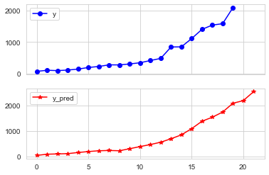
fig = data[['y','y_pred']].plot(subplots = True, style=['b-o','r-*'])
plt.show()
F:\Anaconda\envs\my\lib\site-packages\sklearn\svm\_base.py:1225: ConvergenceWarning: Liblinear failed to converge, increase the number of iterations.
  warnings.warn(
C:\Windows\Temp\ipykernel_63584\2363168573.py:6: FutureWarning: As the xlwt package is no longer maintained, the xlwt engine will be removed in a future version of pandas. This is the only engine in pandas that supports writing in the xls format. Install openpyxl and write to an xlsx file instead. You can set the option io.excel.xls.writer to 'xlwt' to silence this warning. While this option is deprecated and will also raise a warning, it can be globally set and the warning suppressed.
  data.to_excel(outputfile)


真实值与预测值分别为:
           y       y_pred
0     64.87    37.302597
1     99.75    83.928503
2     88.11    94.774134
3    106.07   106.434331
4    137.32   151.059897
5    188.14   188.205356
6    219.91   219.566685
7    271.91   230.340346
8    269.10   219.659959
9    300.55   300.550000
10   338.45   383.515443
11   408.86   463.222420
12   476.72   554.905404
13   838.99   691.434167
14   843.14   843.095183
15  1107.67  1088.163763
16  1399.16  1379.593271
17  1535.14  1536.823098
18  1579.68  1739.224541
19  2088.14  2086.022177
20      NaN  2188.120305
21      NaN  2539.228245